“Ice and Stone 2020” participants have undoubtedly noticed that I have often discussed how this-or-that comet or asteroid will be returning to the inner solar system or passing by Earth at some point in the future, and perhaps have wondered how such things are determined. In principle, the processes by which such events are calculated are relatively straightforward, although as is usually true in many other scientific disciplines – and, indeed, life as a whole – the reality can be considerably more complex. With modern computer technology, this can nevertheless be performed with relative ease, and the results are considerably more accurate than they were in earlier times – although a small bit of uncertainty is always present.
Once a new object is discovered, the first priority is the measurement of its position – i.e., its celestial coordinates of right ascension and declination – with respect to background stars, a practice called “astrometry.” In theory, this can be performed with the unaided eye, and indeed this was the case prior to the invention of the telescope; the 16th-Century Danish astronomer Tycho Brahe could do so with an accuracy of an arcminute, and indeed it was from his astrometric measurements of the planets, Mars in particular, that his protégé Johannes Kepler derived his Three Laws of Planetary Motion. Before the development of astrophotography astrometry was often performed by the usage of a device called a “filar micrometer” that was inserted within the eyepiece of a telescope, but once astrophotography came into its own during the latter part of the 19th Century astrometric measurements could be performed from photographs. With modern electronic devices like charge-coupled devices, i.e., CCDs, and specially-designed software it is now possible to perform astrometric measurements to a high degree of precision and accuracy, to well within an arcsecond.
An astrometric measurement can only be as good as the stars’ positions from which it is measured. The development of accurate star catalogs is thus an important part of this overall process, and this has steadily improved over the years. Until fairly recently stellar positions measured by ESA’s HIgh Precision PARallax COllecting Satellite (Hipparcos) mission – an acronym that references the 2nd Century B.C. Greek astronomer Hipparchus of Nicaea, who performed pioneering work in the measurements of stars – that was launched in 1989 provided the foundation for the best catalogs, but these are now being superseded by measurements from ESA’s Gaia mission (launched in 2013) that ultimately will provide high-accuracy positional determinations for approximately one billion stars. Because of the “wobbling” phenomenon called “precession” – discovered, incidentally, by Hipparchus – and also the fact that the sun and all the other stars are in constant motion with respect to each other, star catalogs need to be referenced to a specific date in time. At present this is the beginning of the year 2000, although presumably within a couple of decades this will shift to 2050.
One other significant issue that arises in astrometric measurements is parallax. Measurements are, for obvious reasons, not made from the center of the earth, but rather from various locations on Earth’s surface, and this can affect an object’s measured position, especially in the case of an object near Earth. Observatories and institutions that have demonstrated the successful ability to perform astrometric measurements are assigned an official “Observatory Code” by the IAU’s Minor Planet Center, which lists each site’s “parallax factors” based upon its latitude, longitude, and altitude above sea level. Although I no longer perform astrometric measurements from my home site, when I was doing so during the early 2000s my Observatory Code was 921.
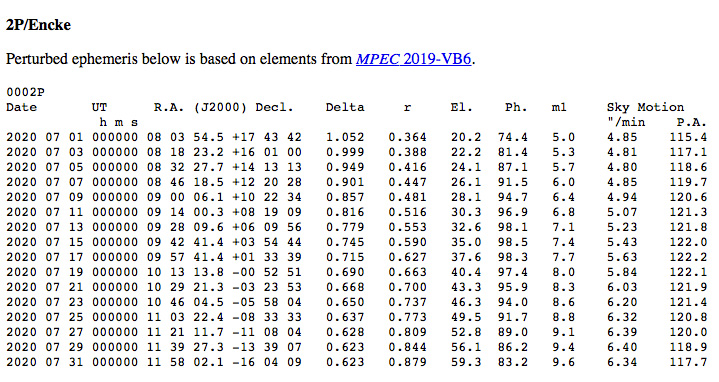
Once astrometric measurements are obtained, an orbit can be calculated from these. Then, after an orbit is determined, it is possible to compute an “ephemeris” (plural “ephemerides”), i.e., a list of appropriate celestial coordinates that the object will occupy at various points in time. In this procedure, the object’s location in its orbit at the time in question is determined, and then the earth’s location in its orbit is determined for the same time, and via a coordinate transformation the object’s sun-centered location is transferred to an Earth-centered location. With the application of a site’s parallax factors it is possible to calculate an ephemeris for a specific geographical location on Earth (or in space, for that matter).
An orbit is defined by various terms called “elements” that describe an orbit’s size, shape, and orientation, and there is also a time element involved. One of the orbital elements is the “inclination,” i.e., how steeply the orbit is inclined with respect to the plane of the earth’s orbit (otherwise known as the “ecliptic”). An orbital inclination of 0 degrees is in the same plane as the ecliptic, whereas an inclination of 90 degrees is exactly perpendicular to the ecliptic. Inclinations greater than 90 degrees (up to 180 degrees) are “retrograde,” i.e., an object in such an orbit travels around the sun in the direction opposite that of Earth.
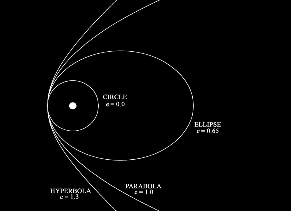
Another important orbital element is the “eccentricity” (usually written as “e”) which in general terms describes the shape of the orbit. An orbit with an eccentricity of 0 is a circle, whereas eccentricity values between 0 and 1 are ellipses, with the higher the eccentricity indicating a more elongated orbit. An eccentricity of exactly 1 is a parabola, and an eccentricity greater than 1 is a hyperbola. Objects in parabolic and hyperbolic orbits are unbounded, i.e., they will never return to the inner solar system, whereas objects in elliptical and circular orbits are bounded and will return after a period of time. (Obviously, objects in circular orbits remain the same distance from the sun all the time.) The highest eccentricity ever observed in a natural object is the recent interstellar Comet 2I/Borisov I/2019 Q4 – a future “Comet of the Week” – which has an orbital eccentricity of 3.4.
The calculation of an orbit follows directly from Newton’s Law of Universal Gravitation, although in the pre-computer era this was mathematically laborious. In principle, an orbit can be calculated from three positions, however in practice, since each position has some error associated with it the more positions that are available, the better-determined the orbit. Orbits based on only a few positions and/or over a short arc can be “indeterminate,” i.e., any number of widely disparate orbits can be fit through the available measurements. As more and more astrometric measurements become available and as the observation arc becomes longer, the “true” orbit begins to emerge, although this is always subject to refinement as more data is collected. It sometimes happens that, once a reasonably valid orbit is determined, “pre-discovery” images of the object in question may be identified weeks or months after the fact, thus allowing for a much more accurate orbit to be calculated. An example of this is Comet Hale-Bopp C/1995 O1 (a future “Comet of the Week”); once the first reasonably good orbits were calculated, a pre-discovery image on a photograph taken over two years earlier allowed the determination of a very solid orbit.
If the sun and the orbiting object were the only objects in the universe, the object would remain on that same orbit indefinitely. Of course, there are many other objects around, primarily the various planets, including – especially – Jupiter, and each of these objects exerts a gravitational pull that perturbs the object and affects its orbit accordingly. (Indeed, numerous comets have approached closely to Jupiter and have had their orbits dramatically affected, some of these even ejected from the solar system altogether on hyperbolic orbits.) While the solution of the “two-body” problem is relatively straightforward, it turns out that there is no analytical solution to the “three-body” or “general n-body” problem; the calculation of orbits that properly involves these perturbing effects can only be performed numerically. Again, back in the pre-computer days this was an extremely laborious process mathematically but is now accomplished via computers with relative ease. Such orbits are called “osculating” orbits and are referenced to a specific date called the “osculation epoch;” in real terms, such an orbit is the one that the object in question is traveling in at that specific point in time.
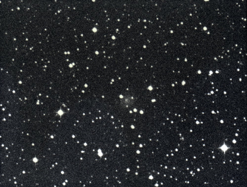
Other effects can appear as well. Comets eject material from their nuclei in jet-like geysers that act as small rocket engines that push the nuclei in the opposite direction; this effect is described under the term “non-gravitational forces” and these were first detected in Comet 2P/Encke, this week’s “Comet of the Week.” Each comet is different, and sometimes the same comet will exhibit different non-gravitational forces at different times, and thus these can only be determined empirically. Small asteroids, in particular, can experience something called the “Yarkovsky-O’Keefe-Radzievskii-Paddack,” or “YORP,” effect, wherein sunlight striking different sides of the asteroid and its own resulting thermal emission can affect its rotation and thus introduce small changes in its orbit. Astrometric measurements of objects near the sun, and the orbits of the objects themselves, can also be affected by General Relativity.
Once all the various effects are allowed for inasmuch as the available data will permit, it is now possible to make predictions for where an object will be in the future. For main-belt asteroids, which generally travel in low-inclination nearly-circular orbits, this is a relatively straightforward process, and once an asteroid has been observed at a few successive oppositions its orbit can be considered “safe” and it can be assigned a permanent number. (The designation and numbering processes are described in a previous “Special Topics” presentation.)
The first predicted return of a periodic comet is somewhat more uncertain, in part because of unknown non-gravitational forces, and it is not unusual for a predicted time of perihelion passage to be off by up to a day or so. (In the pre-computer era, predicted perihelion times could be off by up to several weeks.) Once a comet has been observed on a second return it can then receive a permanent number.
The situation is similar with respect to near-Earth asteroids. These tend to be relatively small objects and are often only detectable when they are relatively close to Earth, and thus several returns may elapse before they are recovered; it is not unusual for first-time recoveries to be off by a few days or more. As with the other objects, once a near-Earth asteroid has been well observed enough such that its orbit can be considered “safe,” it can be assigned a permanent number.
Even the orbits of objects – especially periodic comets and near-Earth asteroids – that are considered “safe” and that are numbered can only be considered “safe” for a few centuries or, at most, a few millennia. The uncertainties in even the best-determined orbits propagate and grow larger over time, and objects can drift into and out of “resonances” with planets such as Jupiter (i.e., an object in 3:2 resonance with Jupiter will orbit the sun three times for every two orbits that Jupiter makes). The orbits of the centaurs – discussed in a previous “Special Topics” presentation – are unstable over a timescale of millennia, and over timescales of tens to hundreds of millions of years, the orbits of all the planets are unstable. For example, numerical simulations have shown a tiny but nevertheless real chance that Mercury could be ejected from the solar system, or could strike the sun, or Venus – or even Earth – sometime with the next few billion years. The upshot of all this is that the solar system we see now, including all the various “small bodies” that are the focus of “Ice and Stone 2020,” is a transient thing, just like everything else in life.
More from Week 26:
This Week in History Comet of the Week Free PDF Download Glossary
Ice and Stone 2020 Home Page
